`\color{red} ✍️` We know that statistics deals with data collected for specific purposes. We can make decisions about the data by analysing and interpreting it.

`\color{red} ✍️` In earlier classes, we have studied methods of representing data graphically and in tabular form.

`\color{red} ✍️` This representation reveals certain salient features or characteristics of the data. We have also studied the methods of finding a representative value for the given data. `color(vlue)("This value is called the measure of central tendency. ")`

Recall mean (arithmetic mean), median and mode are three measures of central tendency.

`\color{red} ✍️` A measure of central tendency gives us a rough idea where data points are centred. But, in order to make better interpretation from the data, we should also have an idea how the data are scattered or how much they are bunched around a measure of central tendency.

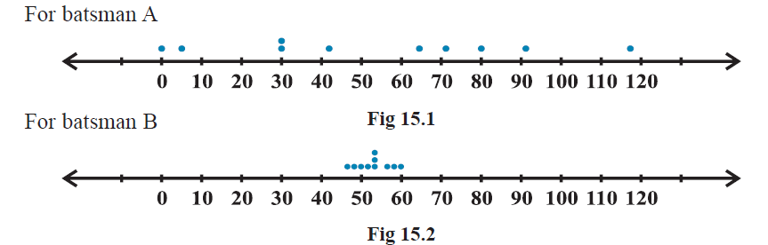
`color(red)(=>"Consider now the runs scored by two batsmen")` in their last ten matches as follows:

`color{orange}("Batsman A" : 30, 91, 0, 64, 42, 80, 30, 5, 117, 71)`

`color{orange}("Batsman B" : 53, 46, 48, 50, 53, 53, 58, 60, 57, 52)`

Clearly, the mean and median of the data are

`color{navy}(\ \ \ \ \ \ \ \ \ \ \ "Batsman A" \ \ \ \ \ \ \ \ \ \ \ "Batsman B")`

`color{orange}("Mean" \ \ \ \ \ \ \ \ \ \ 53\ \ \ \ \ \ \ \ \ \ \ \ \ \ \ \ \ 53)`

`color{orange}("Median" \ \ \ \ \ \ \ \ \53\ \ \ \ \ \ \ \ \ \ \ \ \ \ \ \ \ 53)`

Recall that, we calculate the mean of a data (denoted by `color(blue)(barx)` ) by dividing the sum of the observations by the number of observations, i.e

`color{blue}(barx = 1/n sum_(i=1)^(n) x_i)`

Also, the median is obtained by first arranging the data in ascending or descending order and applying the following rule.

`\color{red} ✍️` If the number of observations is odd, then the median is `color{orange}(((n+1)/2)^(th))` observation.

`\color{red} ✍️` If the number of observations is even, then median is the mean of `color{orange}((n/2)^(th))` and `color{orange}(((n+1)/2)^(th))` observations.

`\color{red} ✍️` We find that the mean and median of the runs scored by both the batsmen `A` and `B` are same i.e., `53.` Can we say that the performance of two players is same?

Clearly No, because the variability in the scores of batsman `A` is from `0` (minimum) to `117` (maximum).

Whereas, the range of the runs scored by batsman `B` is from `46` to `60`.

Let us now plot the above scores as dots on a number line. We find the following diagrams:

`\color{red} ✍️` We can see that the dots corresponding to batsman `B` are close to each other and are clustering around the measure of central tendency (mean and median), while those corresponding to batsman `A` are scattered or more spread out.

`\color{red} ✍️` Thus, the measures of central tendency are not sufficient to give complete information about a given data.

`\color{red} ✍️` Variability is another factor which is required to be studied under statistics. Like ‘measures of central tendency’ we want to have a single number to describe variability. This single number is called a ‘measure of dispersion’.

`\color{red} ✍️` In this Chapter, we shall learn some of the important measures of dispersion and their methods of calculation for ungrouped and grouped data.

The dispersion or scatter in a data is measured on the basis of the observations and the types of the measure of central tendency, used there. There are following measures of dispersion:

`(i)` Range, `(ii)` Quartile deviation, `(iii)` Mean deviation, `(iv)` Standard deviation.

In this Chapter, we shall study all of these measures of dispersion except the quartile deviation.

`\color{fuchsia} {ul ★ "Range"}`

We find the difference of maximum and minimum values of each series. This difference is `color(blue)("called the ‘Range’ of the data.")`

Thus, `color(red)("Range of a series = Maximum value – Minimum value. ")`

`\color{red} ✍️` Recall that, in the example of runs scored by two batsmen A and B, we had some idea of variability in the scores on the basis of minimum and maximum runs in each series. To obtain a single number for this,

In case of `color(navy)("batsman A,")` `color{orange}("Range" = 117 – 0 = 117)` and for `color(navy)("batsman B,")` `color{orange}("Range" = 60 – 46 = 14.)`

Clearly, `color(navy)("Range of A > Range of B.")` Therefore, the scores are scattered or dispersed in case of `A` while for `B` these are close to each other.

`\color{red} ✍️` The range of data gives us a rough idea of variability or scatter but does not tell about the dispersion of the data from a measure of central tendency. For this purpose, we need some other measure of variability. Clearly, such measure must depend upon the difference (or deviation) of the values from the central tendency.

`\color{red} ✍️` The important measures of dispersion, which depend upon the deviations of the observations from a central tendency are mean deviation and standard deviation. Let us discuss them in detail.

`color{green} ✍️` Recall that the deviation of an observation `x` from a fixed value ‘a’ is the difference `color{orange}(x – a.)`

In order to find the dispersion of values of `x` from a central value ‘a’ , we find the deviations about `a.`

An absolute measure of dispersion is the mean of these deviations.

To find the mean, we must obtain the sum of the deviations.

But, we know that a measure of central tendency lies between the maximum and the minimum values of the set of observations.

Therefore, some of the deviations will be negative and some positive. Thus, the sum of deviations may vanish.

Moreover, the sum of the deviations from mean `color{orange}(( barx ))` is zero.

Also `color{blue}(\ \ \ \ \ \ \ \ \ \ \ \ \ \ "Mean of deviations" = ("Sum of deviations")/("Number of observations") = 0/n = 0)`

Thus, finding the mean of deviations about mean is not of any use for us, as far as the measure of dispersion is concerned.

`color{green} ✍️` Remember that, in finding a suitable measure of dispersion, we require the distance of each value from a central tendency or a fixed number `‘a’.`

Recall, that the absolute value of the difference of two numbers gives the distance between the numbers when represented on a number line.

Thus, to find the measure of dispersion from a fixed number `‘a’` we may take the mean of the absolute values of the deviations from the central value. This mean is called the `color(blue)("‘mean deviation’.")`

Thus mean deviation about a central value `‘a’` is the mean of the absolute values of the deviations of the observations from `‘a’.`

The mean deviation from `‘a’` is denoted as `M.D. (a).` Therefore,

`color{blue}(M.D.(a) = ("Sum of absolute values of deviations from 'a'")/("Number of observations"))`

`color{orange}("Remark : ")` Mean deviation may be obtained from any measure of central tendency. However, mean deviation from mean and median are commonly used in statistical studies.

Let us now learn how to calculate mean deviation about mean and mean deviation about median for various types of data

Let `n` observations be `color{blue}(x_1, x_2, x_3, ...., x_n.)`

The following steps are involved in the calculation of mean deviation about mean or median:

`color{red}("Step 1 : ")` Calculate the measure of central tendency about which we are to find the mean deviation. Let it be `‘a’.`

`color{red}("Step 2 : ")` Find the deviation of each `color{blue}(x_i)` from `color{blue}(a)`, i.e., `color{green}(x_1 – a, x_2 – a, x_3 – a,. . . , x_n– a)`

`color{red}("Step 3 : ")` Find the absolute values of the deviations, i.e., drop the minus sign `(–)`, if it is there i.e., , `color{blue}(|x_1-a_1|,|x_2-a|,|x_3-a|,....,|x_n-a|)`

`color{red}("Step 4 : ")` Find the mean of the absolute values of the deviations. This mean is the mean deviation about `color{blue}(a)`, ie..,

`color{blue}(M.D (a) = {sum_(i=1)^(n) |x_1-a|) /n} `

`color{green}(M.D (barx)= 1/n * sum_(i=1)^(n) |x_1-barx|) ` where `color{orange}(barx =)` Mean

Thus `color{navy}(M.D (barx) = 1/n sum_(i=1)^(n) |x_i -M|, \ \ ) ` where `color{orange}(M)` = Median

We know that data can be grouped into two ways :

`color(red)((a))` `color(blue)(" Discrete frequency distribution,")`

`color(red)((b))` `color(blue)(" Continuous frequency distribution.")`

Let us discuss the method of finding mean deviation for both types of the data.

`color{red}("(a) Discrete frequency distribution")`

Let the given data consist of n distinct values `color{orange}(x_1, x_2, ..., x_n)` occurring with frequencies `color{orange}(f_1, f_2 , ..., f_n)` respectively.

This data can be represented in the tabular form as given below, and is `color(blue)("called discrete frequency distribution :")`

`color{orange}(x : " " x_1" "x_2" "x_3 ........ x_n)`

`color{orange}(f : " " f_1" "f_2" " f_3 ........ f_n)`

`color{red}("(i) Mean deviation about mean")`

First of all we find the mean `color(blue)(barx)` of the given data by using the formula

`color{orange}(barx = (sum_(i=1)^(n) x_i f_i)/(sum_(i=1)^(n)f_i) = 1/N sum_(i=1)^(n) x_i f_i,)`

where `color{navy}(sum_(i=1)^(n) x_i f_i,)` denotes the sum of the products of observations `x_i` with their respective frequencies `color{orange}(f_i)`

and `color{navy}(N = sum_(i=1)^(n) x_i f_i,)` is the sum of the frequencies.

Then, we find the deviations of observations `x_i` from the mean `barx` and take their absolute values, i.e., `color{orange}(|x_i - bar x|)` for all `i =1, 2,..., n.`

After this, find the mean of the absolute values of the deviations, which is the required mean deviation about the mean. Thus

`color{blue}(M.D .(barx) = (sum_(i=1)^(n) f_i|x_i-barx|)/(sum_(i=1)^(n) f_i) = 1/N * sum_(i=1)^(n) f_i|x_i - barx|)`

`color{red}("(ii) Mean deviation about median")`

To find mean deviation about median, we find the median of the given discrete frequency distribution.

For this the observations are arranged in ascending order. After this the cumulative frequencies are obtained. Then, we identify the observation whose cumulative frequency is equal to or just greater than `color{orange}(N/2)` N is the sum of frequencies. This value of the observation lies in the middle of the data, therefore, it is the required median. After finding median, we obtain the mean of the absolute values of the deviations from median.Thus,

`color{blue}(M.D .(M) = 1/N sum_(i=1)^(n) f_i |x_i - M|)`

`color{red}((b) "Continuous frequency distribution")`

A continuous frequency distribution is a series in which the data are classified into different class-intervals without gaps along with their respective frequencies.

For example, marks obtained by `100` students are presented in a continuous frequency distribution as follows :



`color{red}((i) "Mean deviation about mean")`

While calculating the mean of a continuous frequency distribution, we had made the assumption that the frequency in each class is centred at its mid-point.

Here also, we write the mid-point of each given class and proceed further as for a discrete frequency distribution to find the mean deviation.

`color{red}((ii) "Mean deviation about median")`

The process of finding the mean deviation about median for a continuous frequency distribution is similar as we did for mean deviation about the mean.

The only difference lies in the replacement of the mean by median while taking deviations.

Let us recall the process of finding median for a continuous frequency distribution. The data is first arranged in ascending order. Then, the median of continuous frequency distribution is obtained by first identifying the class in which median lies (median class) and then applying the formula

`color{blue}("Median" = l + (N/2-C)/fxxh)`

where median class is the class interval whose cumulative frequency is just greater than or equal to `color{orange}((N/2),N)` is the sum of frequencie `color{orange}( l , f , h)` and `color{orange}(C)` are, respectively the lower limit , the frequency, the width of the median class and C the cumulative frequency of the class just preceding the median class.

After finding the median, the absolute values of the deviations of mid-point `color{orange}(x_i)` of each class from the median i.e., `color{orange}(|x_i - M|)` are obtained.

Then `color{blue}(M.D. (M) = 1/N sum_(i=1)^(n) f_i |x_i-M|)`